The Applied ML Workflow

Why notebook ML is not production ML

You've trained models. You've seen a good test accuracy. You've called it done. And then nothing works in the real world.

This gap — between what looks good in a notebook and what holds up in production — is where applied ML begins. The goal of this course is to close it.

Before we get into techniques, let's name the five most common places ML projects fail. None of them are algorithmic.

1. Wrong success metric. The model is optimised for accuracy, but the business cares about minimising false negatives. These are different objectives. Accuracy on a fraud dataset can be 99.9% by predicting nothing is fraud. That model is useless.

2. No baseline comparison. A model that achieves 87% accuracy sounds good — until you discover that always predicting the majority class achieves 85%. Your model added almost nothing.

3. Leaking labels. A feature derived from the target, or future information visible at training time, inflates your validation metrics. The model looks great until it sees real data.

4. Training/serving skew. The preprocessing you ran interactively in the notebook is not exactly replicated at inference time. Columns are in a different order. A scaler was fit on slightly different data. The predictions drift.

5. No monitoring plan. Models degrade as the world changes. Without tracking prediction distributions and outcome rates, you won't know until customers complain.

These aren't advanced problems. They're the standard failure modes of ML work at every level. You'll encounter each one in this course — and learn to catch them before they matter.

The six-stage workflow

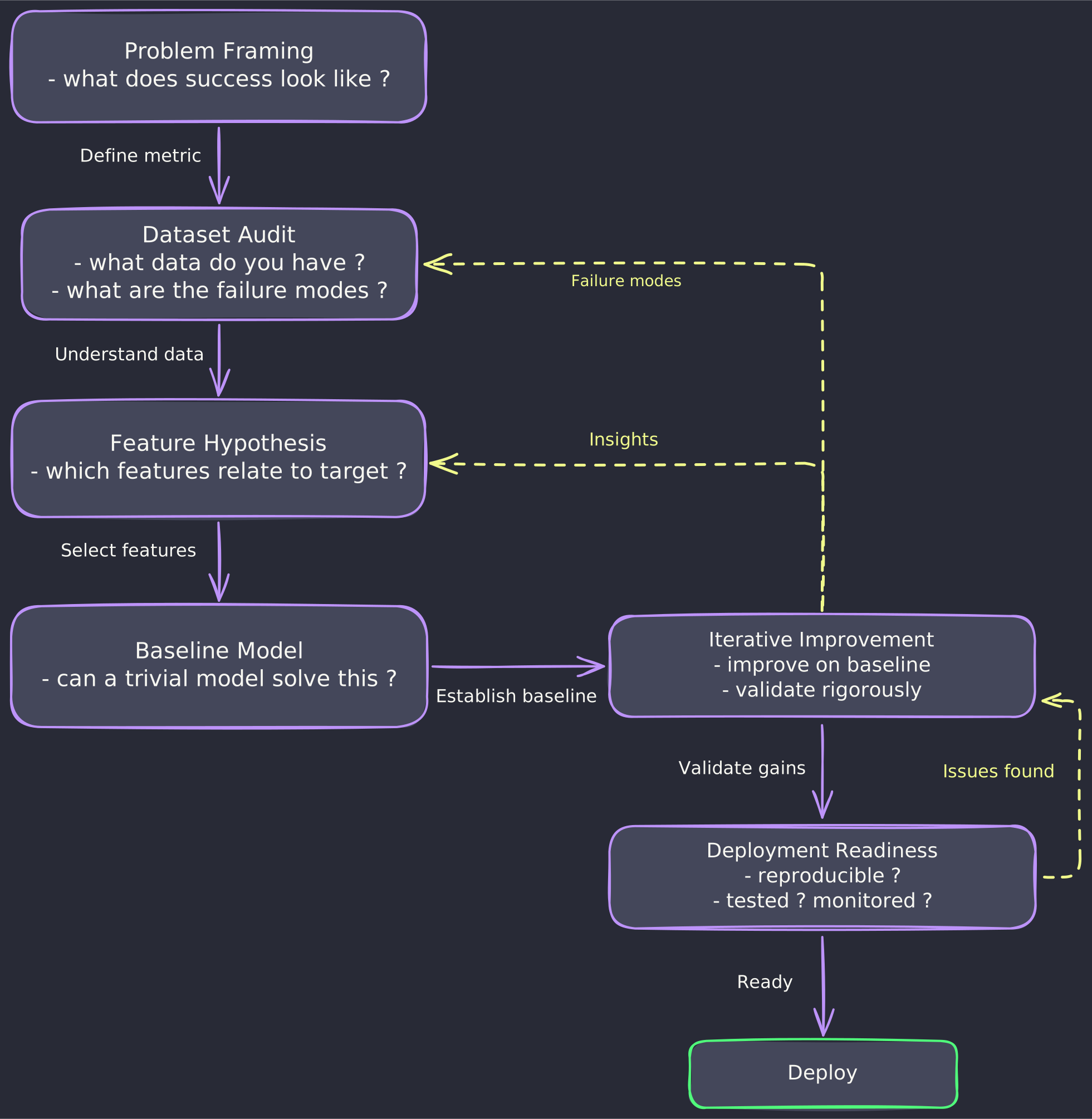
Every production ML project, regardless of domain or algorithm, follows the same loop:

1. Problem framing     → What does success look like, measured how?
2. Dataset audit       → What data do you have, and what are its failure modes?
3. Feature hypothesis  → Which features plausibly relate to the target, and why?
4. Baseline model      → Can a trivial model already solve most of the problem?
5. Iterative improvement → Improve on the baseline; validate rigorously
6. Deployment readiness → Is the pipeline reproducible, tested, and monitored?

This is a loop, not a waterfall. You'll move between stages as you learn more. But starting with a baseline — stage 4 — before investing heavily in feature engineering or model selection is the single most important professional habit this course reinforces.

The baseline-first rule

Before claiming your model is good, you need to know what "good" means relative to doing nothing. That means fitting a naive predictor first.

Scikit-learn's DummyClassifier gives you this in three lines:

from sklearn.dummy import DummyClassifier
from sklearn.metrics import accuracy_score, roc_auc_score

dummy = DummyClassifier(strategy="most_frequent")
dummy.fit(X_train, y_train)
y_pred_dummy = dummy.predict(X_test)
print(f"Dummy accuracy: {accuracy_score(y_test, y_pred_dummy):.3f}")

# Output
Dummy accuracy: 0.927

Now fit your real model:

from sklearn.linear_model import LogisticRegression

model = LogisticRegression(max_iter=1000, random_state=42)
model.fit(X_train, y_train)
y_pred = model.predict(X_test)
print(f"Logistic regression accuracy: {accuracy_score(y_test, y_pred):.3f}")

# Output
Logistic regression accuracy: 0.931

That 0.931 looked impressive until you saw 0.927. The logistic regression is barely outperforming the strategy "always predict the majority class." On this dataset — a loan default prediction task where 92.7% of loans don't default — accuracy is the wrong metric entirely.

This is the baseline doing its job: surfacing a measurement problem before you waste days on feature engineering.

Choosing the right metric at the start

The baseline check also forces the question: what metric should we actually be optimising?

For the loan default example:

• Missing a default (false negative) means the bank loses money
• Incorrectly flagging a healthy loan (false positive) means a customer is denied credit

These have different business costs. The metric should reflect the cost ratio. Accuracy doesn't.

A practitioner decision rule:

• Balanced classes, equal costs → accuracy, macro F1
• Imbalanced classes → AUC-ROC, average precision, F1 on the minority class
• Asymmetric costs → precision/recall tradeoff; threshold tuning (Lesson 4)
• Probability output matters → AUC-ROC, Brier score, calibration (Lesson 8)

You don't need to memorise this table. You need to ask the question before training anything: what does a correct prediction save or cost, relative to an incorrect one?

What this course builds

Each lesson in this course solves a real failure mode:

Lesson	Failure mode addressed
2 — Statistical thinking for evaluation	"The model improved by 2% — is that real?"
3 — Feature selection	"More features made the model worse"
4 — Handling imbalanced data	"The model just predicts the majority class"
5 — Random forests in depth	"Feature importance gave me a nonsense ranking"
6 — Gradient boosting	"The model overfit with too many estimators"
7 — Cross-validation and leakage	"The CV score was great but test was much lower"
8 — Calibration	"The probabilities don't match actual outcomes"
9 — SHAP interpretability	"I can't explain why the model made this prediction"
10 — Production pipelines	"The model works in the notebook but not in the API"

Summary

Applied ML starts before the algorithm. The three questions to answer before touching a model:

1. What metric defines success — and does it reflect the actual business cost of errors?
2. What does a naive baseline score on that metric?
3. What is the minimum improvement over the baseline that justifies shipping?

The rest of this course is about building the skills to answer those questions rigorously and to build models that actually close the gap.

Next: Lesson 2 puts statistical rigour behind model metrics — so you can tell whether a score difference is real or just luck of the split.