Tensors and Autograd

Why PyTorch tensors aren't just NumPy arrays

If you've used NumPy, you already know how to think about multi-dimensional arrays. PyTorch tensors look similar on the surface — same indexing syntax, similar creation functions — but they carry two capabilities that NumPy arrays don't have: device placement and gradient tracking.

Device placement means a tensor can live in GPU memory, not just CPU memory. You can move a tensor to a CUDA device with .to("cuda") and all subsequent operations on it run on the GPU. The data doesn't bounce back to CPU unless you explicitly ask it to. This is what makes training neural networks on GPUs practical without you having to manage memory transfers by hand.

Gradient tracking means PyTorch can watch every operation you perform on a tensor and, at the end of a forward pass, automatically compute the gradient of any scalar output with respect to any input. This is the autograd system, and it's what makes backpropagation invisible to write — you define the forward computation, call .backward(), and the gradients appear.

These two features are why PyTorch tensors exist as a separate type. They're not a drop-in replacement for NumPy; they're a different tool built for a different job.

---

Creating tensors

You'll create tensors constantly. These four constructors cover most situations:

import torch

# From a Python list — dtype is inferred
weights = torch.tensor([0.2, 0.5, 0.3])
print(weights.dtype)   # torch.float32
print(weights.shape)   # torch.Size([3])

# Zeros and ones — specify shape as separate args or a tuple
hidden_state = torch.zeros(4, 128)   # shape (4, 128)
bias = torch.ones(128)               # shape (128,)

# Random normal — standard normal, mean 0, std 1
kernel = torch.randn(64, 3, 3, 3)   # shape (64, 3, 3, 3)
print(kernel.dtype)   # torch.float32
print(kernel.device)  # cpu

A few things to notice. torch.tensor() copies the data from the Python object you pass in. The default floating-point dtype is float32, not float64 — this matters because most GPU operations are optimised for 32-bit. You can override it with the dtype argument: torch.tensor([1.0, 2.0], dtype=torch.float64).

Shapes are reported as torch.Size objects, but they behave like tuples. You'll use .shape constantly when debugging shape mismatches.

---

The computation graph

When requires_grad=True is set on a tensor, PyTorch starts recording every operation that touches it. The result is a computation graph — a directed acyclic graph where each node is a tensor and each edge represents a function that produced it.

The graph is built dynamically, during the forward pass. There's no separate "graph definition" step as in older frameworks. Every time you run your forward computation, PyTorch constructs the graph fresh. This means the graph can change shape between iterations — useful for variable-length sequences and conditional branches.

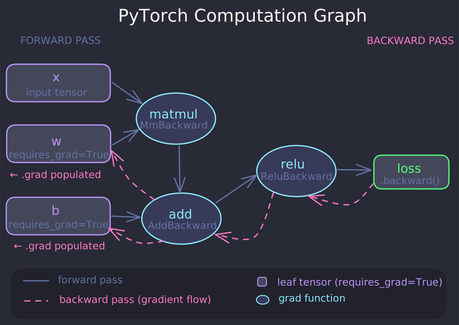
Leaf tensors are the tensors you created directly — your weights, your inputs. Intermediate tensors are the results of operations. When you call .backward(), gradients flow from the output back to the leaves.

---

Autograd and .backward()

You won't write this from scratch — but you need to understand what it does to catch the silent failure it hides.

import torch

# Create two leaf tensors with gradient tracking enabled
x = torch.tensor(3.0, requires_grad=True)
w = torch.tensor(2.0, requires_grad=True)

# Forward pass — PyTorch records every operation
z = w * x + 1.0
loss = z ** 2

# Backpropagation — computes dL/dx and dL/dw
loss.backward()

print(x.grad)   # tensor(48.) — dL/dx
print(w.grad)   # tensor(72.) — dL/dw

After .backward(), each leaf tensor's .grad attribute holds the accumulated gradient of the scalar output with respect to that leaf. The word "accumulated" is important — it's the source of one of the most common bugs in PyTorch training loops.

---

The accumulated gradient trap

Review this code — is it correct?

import torch

x = torch.tensor(3.0, requires_grad=True)
w = torch.tensor(2.0, requires_grad=True)

for step in range(3):
    z = w * x + 1.0
    loss = z ** 2
    loss.backward()
    print(f"Step {step}: w.grad = {w.grad}")

It isn't. Each call to .backward() adds the new gradient to whatever is already stored in .grad. It doesn't replace it. After three steps the gradient in w.grad is three times larger than it should be. In a real training loop this inflates the gradient signal and produces incorrect weight updates.

The fix is to zero the gradients before each backward pass:

for step in range(3):
    if w.grad is not None:
        w.grad.zero_()
    z = w * x + 1.0
    loss = z ** 2
    loss.backward()
    print(f"Step {step}: w.grad = {w.grad}")

In practice, if you're using an optimizer you'll call optimizer.zero_grad() at the top of each training step — that zeros the gradients for every parameter the optimizer manages. The underlying mechanism is exactly the same.

---

Detaching from the graph

Gradient tracking has a cost. PyTorch keeps the computation graph in memory until you release it. When you're running inference or computing metrics, you don't want any of that overhead.

There are two ways to stop tracking.

torch.no_grad() context manager — use this when you want to run a block of code without tracking any operations:

model.eval()

with torch.no_grad():
    predictions = model(validation_inputs)
    val_loss = loss_fn(predictions, validation_targets)

print(val_loss.item())  # .item() extracts the Python float

Inside torch.no_grad(), no computation graph is built, no gradients are computed, and memory usage drops significantly during long validation loops.

.detach() — use this when you want to pull a specific tensor out of the graph while leaving the rest of the computation intact:

# Logging the loss value without keeping the graph alive
loss_value = loss.detach().cpu().numpy()
training_history.append(loss_value)

If you appended loss directly instead of loss.detach(), Python holds a reference to the tensor, and PyTorch keeps the entire computation graph alive for that step. In a long training run, this silently accumulates until you run out of GPU memory.

When logging scalars, .item() is even simpler — it extracts the Python scalar and drops the reference entirely.

---

---

Summary

Tensors are PyTorch's fundamental data structure. What sets them apart from NumPy arrays is device placement — tensors can live on a GPU — and gradient tracking via the autograd system. When requires_grad=True is set, every operation involving that tensor is recorded in a dynamic computation graph. Calling .backward() on a scalar output traverses that graph and deposits gradients in the .grad attribute of each leaf. Gradients accumulate, not replace, so you must zero them before each backward pass. Use torch.no_grad() during inference and validation to avoid building the graph at all, and use .detach() or .item() when you need to extract values for logging.

Next: Lesson 2 covers the full training loop — assembling a Dataset, a DataLoader, an optimizer, and everything you've seen here into a complete model training workflow.