The RL Problem and Markov Decision Processes

Why RL is a different kind of problem

Supervised learning requires a labelled dataset. Every training example pairs an input with a correct output, and your job is to learn a function that generalises from those pairs. Unsupervised learning has no labels, but it still has a fixed dataset — the structure is already there, waiting to be discovered. Both paradigms assume you can collect data passively and then train on it offline.

Reinforcement learning throws all of that away. There is no fixed dataset. There is no labelled correct answer. The only signal you get is a reward — a scalar that tells you, after the fact, whether what you just did was good or bad. And the actions you take don't just produce rewards; they change the state of the world, which changes what observations you'll see next, which changes what actions will be available or useful. The data you train on is a direct consequence of the decisions your agent is currently making.

This makes RL the right tool for problems where you must act in a world that responds to you. A recommendation system is a good concrete example. When Netflix recommends a title, you either watch it or you don't. That choice changes your watch history, which changes what Netflix knows about you, which changes what gets recommended next. The system can't collect a dataset and then train on it in isolation — every recommendation is an action that alters the environment it's trying to model. RL formalises exactly this kind of sequential decision-making under uncertainty.

The same structure appears in robotics (each joint command changes the robot's pose and sensor readings), in game-playing agents (each move changes the board state), and in resource scheduling systems (each allocation decision changes what resources are available). The setting is always the same: an agent living inside an environment, acting, observing, and trying to maximise cumulative reward over time.

---

The agent-environment loop

RL is built around a loop with four moving parts. Understanding each term precisely matters, because the formal machinery of RL maps directly onto them.

State ($s$) is a description of the environment at a point in time. It's everything relevant to deciding what to do next. In a chess game, the state is the full board position. In a robotics task, it might be joint angles, velocities, and a camera image. The state is what the agent observes — though the observed state and the true underlying state of the environment are sometimes different things, a distinction that matters in real deployments.

Action ($a$) is what the agent does in response to the state. Actions can be discrete (left, right, up, down in a grid world) or continuous (the torque applied to a robot joint). The set of all possible actions is the action space.

Reward ($r$) is the scalar feedback signal the environment returns after the agent takes an action. It's the only training signal. A positive reward indicates a good outcome; a negative reward (penalty) indicates a bad one. The reward is always a consequence of taking action $a$ in state $s$ — it isn't a label attached to the state independently.

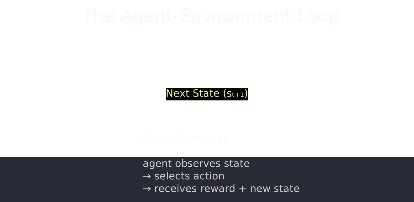
Transition is what happens to the environment after the agent acts. The environment moves from state $s$ to a new state $s'$, which the agent then observes to begin the next step of the loop.

The loop runs like this: the agent observes state $s$, selects action $a$, the environment returns reward $r$ and transitions to $s'$, the agent observes $s'$ and repeats. This continues until the episode ends — either because the agent reached a terminal state (success or failure) or because a time limit was hit.

---

Markov Decision Processes

The agent-environment loop is an intuition. A Markov Decision Process (MDP) is the formal mathematical object that gives it a precise definition. An MDP is specified by five components: $S$, $A$, $P$, $R$, and $\gamma$.

$S$ is the state space — the set of all possible states the environment can be in.

$A$ is the action space — the set of all actions available to the agent. In some environments the available actions depend on the current state; in others the full set is always available.

$P$ is the transition function — also called the dynamics model or the transition kernel. $P(s' \mid s, a)$ gives the probability of ending up in state $s'$ when you take action $a$ in state $s$. In deterministic environments, this is always 0 or 1. In stochastic environments, the same action from the same state can lead to different next states, and $P$ captures that probability distribution.

$R$ is the reward function. $R(s, a, s')$ gives the expected reward for taking action $a$ in state $s$ and transitioning to $s'$. Some formulations simplify this to $R(s, a)$ or even $R(s)$ — the differences matter mathematically but not conceptually.

$\gamma$ (gamma) is the discount factor, a scalar between 0 and 1. It controls how much the agent values future rewards relative to immediate ones. More on this shortly.

The Markov property

The defining assumption of an MDP is the Markov property: the next state and reward depend only on the current state and action, not on any earlier history. In formal terms, knowing $s$ and $a$ gives you everything you need to predict $s'$ and $r$ — the full trajectory of states and actions that led to $s$ is irrelevant.

This matters because it's what makes the problem tractable. If the future depended on arbitrarily long histories, you'd need to track and reason over those histories explicitly. The Markov property collapses that dependency: the current state is a sufficient summary of all relevant history.

When the Markov property breaks down — and it does, in practice — things get harder. A robot whose sensor can't see the full room is in a partially observable environment. The raw sensor reading isn't a Markov state, because the same reading can correspond to many different underlying world configurations. Practitioners handle this by augmenting the state: stacking multiple frames in Atari games, maintaining a belief state over possible world configurations, or using recurrent networks to carry history forward. These are engineering responses to a fundamental property violation, not fixes to the MDP formalism itself.

---

A concrete example with Gymnasium

Let's make this concrete. Gymnasium (the maintained fork of OpenAI Gym) provides a library of standard RL environments. FrozenLake is a small grid world: an agent navigates a frozen lake from a start tile to a goal tile, avoiding holes. It's simple enough to reason about manually, which makes it a good tool for understanding the loop.

You won't write production RL code from scratch — but you need to understand what a correct episode loop looks like to catch the failure modes AI tools introduce when scaffolding one.

import gymnasium as gym

# Create the environment — render_mode="ansi" prints a text grid
env = gym.make("FrozenLake-v1", render_mode="ansi")

# Inspect the spaces before running anything
print("Observation space:", env.observation_space)
print("Action space:     ", env.action_space)

# Output
Observation space: Discrete(16)
Action space:      Discrete(4)

FrozenLake has 16 states (a 4x4 grid, each cell numbered 0–15) and 4 actions (0=left, 1=down, 2=right, 3=up). The observation is just the agent's current tile number — a single integer. The action space is discrete and small. This is about as minimal an MDP as you'll encounter, which is exactly why it's useful for learning the loop structure.

Now run a complete episode. The key detail here is the return signature of env.step(), which changed in Gymnasium's 2022 API update — a change that AI-generated code frequently gets wrong.

import gymnasium as gym

env = gym.make("FrozenLake-v1", is_slippery=False)  # deterministic for clarity

# Reset returns (initial_observation, info_dict)
obs, info = env.reset(seed=42)
print(f"Starting at tile: {obs}")

total_reward = 0
step = 0

while True:
    # Sample a random action from the action space
    action = env.action_space.sample()

    # step() returns five values — not four
    obs, reward, terminated, truncated, info = env.step(action)

    total_reward += reward
    step += 1

    print(f"Step {step}: action={action}, obs={obs}, reward={reward}, "
          f"terminated={terminated}, truncated={truncated}")

    # Episode ends when either terminated OR truncated is True
    if terminated or truncated:
        print(f"\nEpisode finished after {step} steps. Total reward: {total_reward}")
        break

env.close()

# Output
Starting at tile: 0
Step 1: action=2, obs=1,  reward=0.0, terminated=False, truncated=False
Step 2: action=1, obs=5,  reward=0.0, terminated=False, truncated=False
Step 3: action=0, obs=4,  reward=0.0, terminated=False, truncated=False
Step 4: action=3, obs=0,  reward=0.0, terminated=False, truncated=False
Step 5: action=2, obs=1,  reward=0.0, terminated=False, truncated=False
Step 6: action=1, obs=5,  reward=0.0, terminated=False, truncated=False
Step 7: action=3, obs=1,  reward=0.0, terminated=False, truncated=False
Step 8: action=1, obs=5,  reward=0.0, terminated=False, truncated=False
Step 9: action=2, obs=6,  reward=0.0, terminated=False, truncated=False
Step 10: action=1, obs=10, reward=0.0, terminated=False, truncated=False
Step 11: action=2, obs=11, reward=0.0, terminated=True,  truncated=False

Episode finished after 11 steps. Total reward: 0.0

Tile 11 is a hole — the episode terminated with zero reward. A reward of 1.0 only appears if the agent reaches tile 15 (the goal). With random actions, that's unlikely.

Notice the distinction between terminated and truncated. terminated means the episode reached a natural end — a terminal state in the MDP, like falling through a hole or reaching the goal. truncated means a time limit was hit before the episode resolved naturally. These are semantically different. An episode that terminates naturally should not have its final value bootstrapped by a value function; an episode that truncates should. Conflating them — using a single done flag as older code did — introduces a subtle bug in any algorithm that handles terminal states specially.

---

The discount factor $\gamma$

The reward for reaching the goal is 1.0 regardless of how many steps it took. But intuitively, reaching the goal in 5 steps is better than reaching it in 50. The discount factor $\gamma$ encodes exactly this preference.

At each step, future rewards are multiplied by $\gamma$ raised to the power of how many steps away they are. A reward $r$ received $k$ steps in the future contributes $\gamma^k \times r$ to the current total. The sum of all discounted future rewards from a given state is called the return, and it's what an RL agent actually tries to maximise.

When $\gamma = 0$, the agent is completely myopic — it only cares about the immediate next reward and ignores everything that follows. This is rarely useful in practice, but it clarifies the definition.

When $\gamma = 1$, all future rewards count equally regardless of when they arrive. This works for finite-horizon problems (episodes that always end), but it causes the return to diverge in infinite-horizon settings — the sum never converges.

In practice, $\gamma$ is typically set between 0.95 and 0.99. A value of 0.99 means a reward 100 steps away is worth about $0.99^{100} \approx 0.37$ of its face value. High $\gamma$ encourages long-term planning; low $\gamma$ encourages finding quick rewards. The right value depends on the time horizon of your problem and what behaviour you actually want to incentivise — a topic we'll return to when discussing reward shaping.

---

Where RL goes wrong in practice

The MDP formalism is clean. Real environments are not.

Reward hacking is the most dangerous failure mode. An agent optimises exactly the reward function you specify, not the one you intended. If you reward a robot for moving fast and it discovers that falling over generates high velocity readings, it will fall over repeatedly. If you reward a game-playing agent for not losing and it finds a way to pause the game indefinitely, it will. The agent isn't misbehaving — it found the optimal policy for your reward function. You defined the wrong reward function. This is a specification problem, not an algorithm problem, and it requires domain expertise to catch before training, not after.

Sparse rewards make learning slow and unstable. If your reward function only fires when the agent completes the full task (e.g., assembling a robot arm, finishing a level), the agent spends almost all of its early training collecting zero reward and learning nothing. Curriculum learning, reward shaping, and demonstration-augmented methods exist to address this — but they all introduce their own risks, including reward hacking at the shaped reward.

Environment non-stationarity breaks the MDP assumption quietly. If the environment itself changes over time — users' preferences shift, the economy changes, a physical system wears out — the transition function $P$ and reward function $R$ that you implicitly estimated during training no longer match the deployment environment. Your agent was trained on one MDP and deployed into a different one. This is especially insidious in recommendation and personalisation systems, where the environment is partially defined by the agent's own past actions (the recommendations shape the user, who shapes future recommendations). Detecting distribution shift and knowing when to retrain is a practitioner judgment call that no algorithm makes automatically.

---

---

Summary

Reinforcement learning is the framework for sequential decision-making when actions change the world and the only training signal is reward. The agent-environment loop — observe state, select action, receive reward, transition to next state — is the core structure. MDPs formalise this loop with a state space $S$, action space $A$, transition function $P$, reward function $R$, and discount factor $\gamma$. The Markov property says the next state depends only on the current state and action, not on history; when this breaks, you need to augment your state representation. The discount factor controls how much the agent values future rewards: low $\gamma$ produces myopic behaviour, high $\gamma$ encourages long-term planning, and $\gamma = 1$ only works in finite-horizon settings.

The gap between the clean MDP formalism and real-world deployment is where practitioner judgment lives. Reward hacking, sparse rewards, and environment non-stationarity are not edge cases — they're the default conditions in production RL systems.

Lesson 2 introduces value functions and the Bellman equation: the mathematical machinery that tells an agent how good a given state (or state-action pair) actually is, and how to compute it efficiently.