What Makes Time Series Different

A time series is a sequence of observations recorded at successive points in time — daily orders, hourly server load, monthly revenue — where the order of the observations carries information. This lesson explains why the standard machine-learning workflow's core assumption, that rows are independent and interchangeable, fails on temporal data, and why the familiar habits it licenses — shuffling, random train/test splits, cross-validation with arbitrary folds — produce forecasts that score well in evaluation and fail in production.

The assumption you've been relying on

Every course before this one worked with cross-sectional data: one row per customer, per transaction, per image. The rows were assumed to be independent — knowing row 41 tells you nothing about row 42, so you could shuffle them, split them randomly, and average metrics across arbitrary folds.

Time series data breaks that assumption on purpose. Yesterday's order count is the single best predictor of today's. Rows are not interchangeable observations of a population; they are consecutive states of one evolving process. That dependency is not a nuisance to be engineered away — it is the signal you are trying to model.

Order is the information

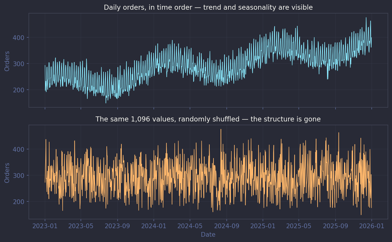
The measurable form of that dependency is autocorrelation: the correlation of a series with a lagged copy of itself. You'll study it properly in Lesson 4, but one number is enough to make the point. This course uses one consistent dataset throughout — three years of daily order counts for an online store — generated synthetically so every example is reproducible:

import numpy as np
import pandas as pd

rng = np.random.default_rng(42)
days = pd.date_range("2023-01-01", "2025-12-31", freq="D")
t = np.arange(len(days))

trend   = 200 + 0.15 * t                                             # slow growth
weekday = np.array([-14, -18, -11, -6, 9, 52, 61])[days.dayofweek]   # weekend peak
yearly  = 38 * np.sin(2 * np.pi * (days.dayofyear - 320) / 365.25)   # holiday-season high
noise   = rng.normal(0, 16, len(days))

orders = pd.Series(trend + weekday + yearly + noise, index=days, name="orders").round()

print(f"lag-1 autocorrelation: {orders.autocorr(lag=1):.3f}")
print(f"lag-7 autocorrelation: {orders.autocorr(lag=7):.3f}")

shuffled = pd.Series(rng.permutation(orders.to_numpy()), index=days)
print(f"lag-1 after shuffling: {shuffled.autocorr(lag=1):.3f}")

lag-1 autocorrelation: 0.786
lag-7 autocorrelation: 0.933
lag-1 after shuffling: -0.004

Consecutive days correlate at 0.786, and days one week apart at 0.933 — the weekly rhythm is even stronger than day-to-day persistence. Shuffle the same 1,096 values and the correlation collapses to zero. The values didn't change; only the order did. Whatever was predictable about this series lived in the ordering.

Three habits that stop working

The broken independence assumption invalidates three specific habits, and each one gets a dedicated fix later in the course:

1. Random train/test splits. A random split scatters test days between training days. The model gets to "predict" a Tuesday while having seen the Monday before it and the Wednesday after it — information no deployed forecast will ever have. This is temporal leakage, the failure mode this course returns to repeatedly, and Lesson 7 replaces random splits with rolling-window backtests.

2. Treating rows as complete. Cross-sectional rows are either present or absent. Time series have a third state: a missing period — a day with no row at all. Aggregations silently skip it, and the gap only becomes visible once the datetime index is handled properly (Lesson 2).

3. Modelling the raw series directly. A series like the one above is really three overlapping signals — trend, seasonality, and everything else. Models, baselines, and sanity checks all get sharper once you can separate them (Lesson 3), and simple baselines built on that structure are surprisingly hard to beat (Lesson 4).

Why this matters more when AI writes the code

AI assistants generate forecasting code fluently — and they reproduce exactly these failures. Ask one to "evaluate a model that predicts daily sales" and there's a good chance you get train_test_split(X, y, test_size=0.2) with its default shuffle=True: syntactically clean, high score, temporally leaked. The generated code runs, the metric looks strong, and nothing flags that the evaluation answered the wrong question.

That's why this course is structured around judgment rather than recipes. The second half — classical models, ML-based forecasting, backtesting — repeatedly asks one question of every piece of code: at the moment this forecast would be made, is every input already known? By the capstone (Lesson 8) you'll apply that question as a repeatable audit protocol to an AI-generated forecasting pipeline.

Summary

• Time series are ordered observations of one evolving process; the ordering itself carries the predictive information, measured as autocorrelation
• The course dataset (three years of daily orders: trend + weekly seasonality + yearly seasonality + noise) correlates at 0.786 day-to-day and 0.933 week-to-week — shuffling destroys both
• Random splits, shuffle-based cross-validation, and ignoring missing periods are the habits that break; temporal leakage is the failure mode they share
• AI-generated forecasting code reproduces these failures fluently, so the durable skill is auditing temporal correctness, not typing the pipeline

Next lesson: Everything in time series analysis sits on top of a well-formed datetime index. Lesson 2 covers parsing dates, resampling between frequencies, and the silent ways both go wrong in pandas.